Prediction with Tensorflow and Streamlit
Besides the actual data and the historical trends, I wanted to have some kind of prediction too and a natural choice was to look into Tensorflow framework which is built for Python and provide a lot of handy tools and algorithms. In this post I’ll talk a bit about the technical stuff and some analysis from the results.
Coding
I’m somewhat rusty from the ML classes in the university, but no problem as there good tutorials available in the Tensorflow documentation. So I followed the Case Study for atmospheric COs which has a good similarity with our data as it’s seasonal – the weekend effect I mentioned on Analyzing trends - Streamlit and Covid BR. The result was pretty much the code below
trend = tfp.sts.LocalLinearTrend(observed_time_series=data_tf)
seasonal = tfp.sts.Seasonal(num_seasons=14,
                            num_steps_per_season=1,
                            observed_time_series=data_tf)
model = tfp.sts.Sum([trend, seasonal], observed_time_series=data_tf)

variational_post = tfp.sts.build_factored_surrogate_posterior(model=model)
num_variational_steps = 200
optimizer = tf.optimizers.Adam(learning_rate=.1)
tfp.vi.fit_surrogate_posterior(target_log_prob_fn=model.joint_log_prob(observed_time_series=data_tf),
                               surrogate_posterior=variational_post,
                               optimizer=optimizer,
                               num_steps=num_variational_steps)
samples = variational_post.sample(100)

forecasted_num = 30
days = pd.date_range(start=date.today(), periods=forecasted_num)
forescast_dist = tfp.sts.forecast(model=model,
                                  observed_time_series=data_tf,
                                  parameter_samples=samples,
                                  num_steps_forecast=forecasted_num)
forecasted = forescast_dist.mean().numpy()[..., 0]
However there are some small tweaks that I had to do to make everything work.
Data type
I was using standard float data type in the my Pandas DataFrames, but Tensorflow won’t work properly using this kind of data. So I had first to convert the DataFrame - a Series in fact - to Tensorflow’s data by using a simple command:
data_tf = tf.convert_to_tensor(original_series, tf.float64)
The interesting point is that I didn’t need to convert back. The output from Tensorflow went straight to the chart.
Caching
Calculating the model is costly, specially the variational inference fitting, so I didn’t want to have it recalculating every time. Happily, Streamlit provides a decorator for caching. Basically it won’t call the decorated method unless there was some change in the input data or in the methods own code. This way, the application will only calculate the model for a given configuration once – what is around once per day/per state.
@st.cache
def _model_and_fit(data):
    ...
It is easy to feel the improvement when playing in the webpage and setting the same state for the second time.
Package size
As I’m using Heroku platform, there is one limitation there regarding the total package size, including the requirements. When first trying to deploy using the base tensorflow package, it went way above Heroku’s limit of 500MB. One solution, the one I adopted, is to use the tensorflow-cpu package, which doesn’t have GPU support but it’s smaller (~300MB less) the the full package, because there will be no GPUs on Heroku for me to be running on anyway.
Analysis
This first predictor is very simple and tends to replicate the last shapes. Though I think it can be reasonable to show where the trend is going.
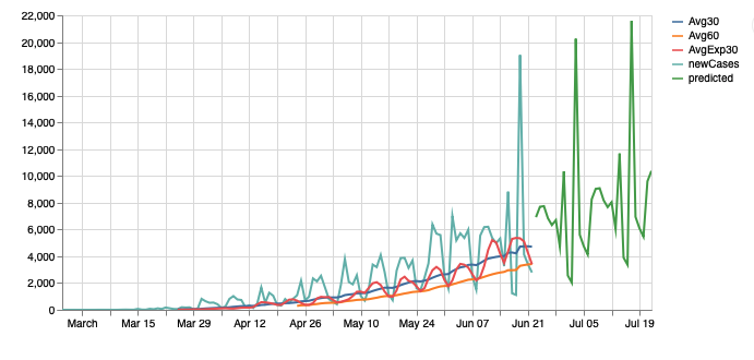
This chart for Sao Paulo shows that the even with all variations, the trend is still up. One interesting detail is that the exponential average is touching the 60-day average, which is now the support and needs to be broken to revert the trend.
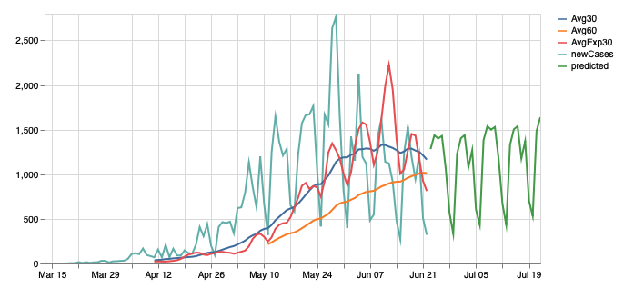
Looking into the Amazonas data, the predicted curve for the next days show stabilization in the trend, going lateral. Which matches the news we are getting that the pressure in the health system has lowered. Just remember that this reflects more the public state of 2 weeks earlier.